Bridging the Gap: Strategies for Overcoming Data Scarcity in AI


What is Data Scarcity in the Context of AI?
Data scarcity in AI refers to the situation where there is an insufficient amount of high-quality data available to train machine learning models effectively. In the development of AI systems, data serves as the foundational fuel that drives learning and prediction. The more data available, the better an AI model can learn from it, identify patterns, and make accurate predictions. However, in many real-world scenarios, collecting, curating, and labelling large datasets is challenging, leading to data scarcity.
Why is Data Scarcity a Significant Challenge?
1. Reduced Model Accuracy : Machine learning models, particularly deep learning models, require extensive datasets to generalize well and achieve high accuracy. These models learn by identifying patterns and relationships in data. When there is a limited amount of data, the model struggles to learn these patterns effectively. Instead of capturing the underlying relationships, the model might only recognize noise or very specific features from the small dataset, leading to poor performance.
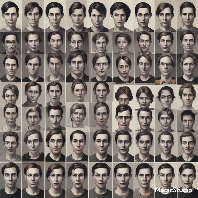
Example: Consider a facial recognition system trained on a dataset of only 100 images of different faces. The model might perform well on these 100 images but will likely fail to generalize to new faces it hasn’t seen before, resulting in lower accuracy when applied to a broader set of images.
2. Overfitting:
Overfitting occurs when a model learns the training data too well, including its noise and outliers, rather than learning general patterns. With a small dataset, a model might memorize the training examples instead of learning to generalize, which means it performs well on training data but poorly on new or unseen data.
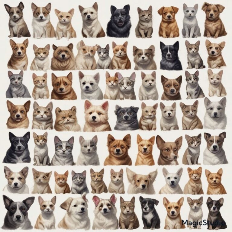
Example: Imagine training a deep learning model to classify images of cats and dogs using only 50 images of each class. The model might achieve perfect accuracy on this limited dataset but fail to correctly classify images of cats and dogs it encounters later because it has not learned the general characteristics of the classes but has memorized specific details from the training images.
Mitigating Reduced Model Accuracy and Overfitting through Data Augmentation
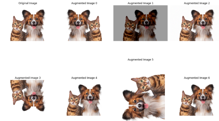
Given the challenges posed by reduced model accuracy and overfitting due to data scarcity, one effective strategy is data augmentation. Data augmentation involves creating variations of your existing dataset by applying transformations such as rotations, flips, or color adjustments. By artificially increasing the size of your dataset, data augmentation helps the model learn more robustly, reducing the risk of overfitting and improving generalization to new data.
Example: Below is a simple code snippet demonstrating how data augmentation can be applied:
import cv2
import albumentations as A
import numpy as np
import matplotlib.pyplot as plt

# Load an example image from a file
def load_image(image_path):
img = cv2.imread(image_path)
if img is None:
raise ValueError("Image not found or unable to load.")
return img

# Define the augmentations
def get_transform(loop):
if loop == 0:
transform = A.Compose([
A.HorizontalFlip(p=1),
])
elif loop == 1:
transform = A.Compose([
A.RandomBrightnessContrast(p=1),
])
elif loop == 2:
transform = A.Compose([
A.GaussNoise(var_limit=(10.0, 50.0), p=1),  # Changed to GaussNoise
])
elif loop == 3:
transform = A.Compose([
A.VerticalFlip(p=1)
])
elif loop == 4:
transform = A.Compose([
A.Blur(blur_limit=(3, 3), p=1)
])
elif loop == 5:
transform = A.Compose([
A.Transpose(p=1)
])
elif loop == 6:
transform = A.Compose([
A.RandomRotate90(p=1)
])
elif loop == 7:
transform = A.Compose([
A.ImageCompression(quality_lower=50, quality_upper=90, p=1)
])
return transform

def augment_and_display_image(image_path):
image = load_image(image_path)

# Ensure image is in RGB format
image = cv2.cvtColor(image, cv2.COLOR_BGR2RGB)

# List to hold augmented images
images = [image]
titles = ['Original Image']

for i in range(8):
img = image.copy()
transform = get_transform(i)
augmented = transform(image=img)
augmented_image = augmented['image']
images.append(augmented_image)
titles.append(f'Augmented Image {i}')

# Display images
plt.figure(figsize=(15, 15))
for i in range(len(images)):
plt.subplot(3, 4, i + 1)
plt.imshow(images[i])
plt.axis('off')
plt.title(titles[i])
plt.tight_layout()
plt.show()

# Example image path (change to a valid local image path)
image_path = '/content/dogcat.jpg'  # Replace with your image file path
augment_and_display_image(image_path)
Output:-
3. Bias in Models:
When dealing with data scarcity, the limited dataset often fails to capture the full diversity of the real-world scenarios the AI model will encounter. As a result, the model may learn patterns that are not representative of the broader population. This can lead to biased predictions where certain groups or scenarios are over- or under-represented.
Example: If a dataset is small and predominantly includes data from one demographic group (e.g., primarily young people or individuals from a specific region), the AI model may perform well for that group but poorly for others. For example, facial recognition systems trained on datasets lacking diversity have been shown to have higher error rates for people with darker skin tones.
4. Challenges in Transfer Learning:
Transfer learning involves using a pre-trained model as a starting point and fine-tuning it on a smaller, task-specific dataset. However, the success of transfer learning depends on having enough relevant data to adapt the pre-trained model to the new task. If the task-specific dataset is too small, even transfer learning might not be effective, and the adapted model might not perform well.
Example: A pre-trained model for image classification on general object categories (like ImageNet) might be adapted for classifying medical images of rare diseases. If the dataset of medical images is very limited, the fine-tuned model might not learn the specific features necessary to accurately identify the diseases, resulting in poor performance.
5. High Cost of Data Collection and Labeling:
Collecting and labeling data can be expensive and labor-intensive, especially in specialized fields like medical imaging or autonomous driving. High costs and resource constraints can limit the amount of high-quality labeled data available, making it difficult to train effective models.
Example: In autonomous driving, collecting labeled data involves capturing numerous hours of driving footage and annotating it with information about road signs, pedestrians, and other vehicles. This process is costly and requires significant human effort, and the scarcity of such high-quality labeled data can hinder the development and performance of self-driving car systems.

1. Collaborative Data Sharing:
Collaborative data sharing involves forming partnerships or agreements between organizations to share data resources. This is particularly valuable in fields like healthcare, where data privacy concerns and regulations often limit data availability. By pooling data, organizations can create larger, more diverse datasets that enhance model performance and generalization.
Example: In the healthcare sector, different hospitals or research institutions might collaborate to share anonymized patient data for developing predictive models for rare diseases. For instance, several hospitals might join forces to create a comprehensive dataset of medical images and patient records, which can be used to train more accurate diagnostic models. This collaboration not only enhances the quality of the data but also helps in overcoming the limitations of individual datasets.
2. Crowdsourcing Data:
Crowdsourcing involves leveraging a large number of people to collect or label data. This method is especially useful when data collection is time-consuming or expensive. Platforms like Amazon Mechanical Turk allow researchers to distribute tasks to a vast number of workers who can perform data annotation or collection tasks, providing a cost-effective solution to gather large volumes of data.
Example: Suppose a company wants to develop a model for detecting offensive language in social media posts. Instead of manually labeling thousands of posts, they can use crowdsourcing platforms to hire workers to annotate the data. By creating specific guidelines and quality control measures, the company can gather a diverse and extensive labeled dataset efficiently, improving the model’s accuracy in detecting offensive language across various contexts and languages.
3.Using Weak Supervision:
Weak supervision involves using noisy, limited, or incomplete sources to generate labeled data. This approach can help build models when high-quality, fully labeled data is scarce. Techniques in weak supervision include using heuristics, external knowledge bases, or semi-supervised learning methods to generate training labels from imperfect sources.
Example: Imagine a scenario where a company wants to train a sentiment analysis model but has only a small set of labeled examples. They might use weak supervision techniques to create additional labeled data. For example, they could employ heuristic rules to label a large number of text samples based on keyword lists or use pre-trained sentiment classifiers to generate pseudo-labels for a larger dataset. This augmented dataset, despite being imperfect, can help train a more robust sentiment analysis model.
Leveraging External Data Sources
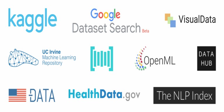
1. Open Datasets:
Open datasets are publicly available collections of data that can be used to supplement proprietary datasets, especially when data is scarce. These datasets span various domains, including healthcare, natural language processing, computer vision, and more. Leveraging open datasets can help improve model performance by providing additional training data, reducing the risk of overfitting, and enhancing generalization.
Examples:
2. Transfer Learning Across Domains:
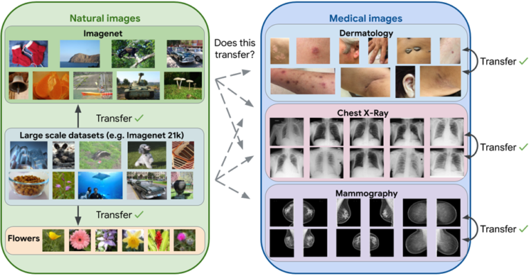
Transfer learning involves taking a pre-trained model from one domain and fine-tuning it on a related but different domain with limited data. This technique is particularly useful when working in specialized areas where collecting large amounts of labeled data is challenging. By leveraging knowledge from a related domain, transfer learning can significantly reduce the amount of data required to achieve good performance.
Examples:· Natural Images to Medical Imaging: Models pre-trained on large datasets of natural images (e.g., ImageNet) have been successfully fine-tuned for medical imaging tasks, such as detecting tumors in X-rays or MRI scans.
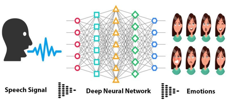
· Speech Recognition to Emotion Detection: A model trained on a large speech recognition dataset can be fine-tuned for emotion detection in speech, where the available data might be limited.
Role of Synthetic Data
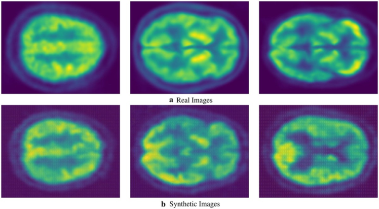
Effectiveness of GANs in Overcoming Data Scarcity: A Case Study in Medical Imaging:
A notable example of the effectiveness of GANs can be found in medical imaging, where GANs have been used to generate realistic PET(positron emission tomography) images for training deep learning models. A research study demonstrated that GAN-generated synthetic PET scans could be used to augment training datasets, enabling the development of models that perform comparably to those trained on real data. This is particularly valuable in the medical field, where privacy concerns and the scarcity of labeled data often hinder model development. The success of this approach highlights how GANs can create valuable data without compromising patient privacy, making them a powerful tool for overcoming data scarcity in sensitive domains like healthcare.
Beyond GANs :
While Generative Adversarial Networks (GANs) are popular for generating synthetic data, other methods like Variational Autoencoders (VAEs) and simulation-based methods offer alternative approaches. VAEs can learn a probabilistic model of the data and generate new samples by sampling from the learned distribution. Simulation-based methods generate data by modeling and simulating real-world processes, making them particularly useful in fields like autonomous driving or robotics.
Examples:
– Simulation-Based Methods: Simulators such as CARLA (Car Learning to Act) and Unity create virtual environments that mimic real-world driving conditions in autonomous driving. These simulators allow developers to generate a wide range of driving scenarios, including weather conditions, traffic patterns, road types, and even rare or dangerous situations that might be difficult or impossible to capture.
Challenges with Synthetic Data
The three major challenges to using synthetic data are:
Should Reflect Reality:
Synthetic data should reflect reality as accurately as possible. However, it is sometimes impossible to generate synthetic data that doesn’t contain elements of personal data. On the flip side, if the synthetic data doesn’t reflect reality, it won’t be able to exhibit patterns necessary for model training and testing. Training your models on unrealistic data doesn’t produce credible insights.
Example: In autonomous driving, a simulator like CARLA is used to generate synthetic driving scenarios. If the simulator accurately reflects real-world conditions—such as different road types, traffic situations, and weather conditions—the synthetic data can be very useful for training and testing autonomous driving systems. For instance, if the simulator includes realistic traffic patterns and road hazards, the model trained on this data is more likely to perform well in real-world driving situations. However, if the synthetic data only includes ideal driving conditions with no variations, the model may struggle when encountering real-world complexities.
Scenario: A model trained on synthetic data with only clear, sunny weather might not perform well in adverse conditions like rain or fog. To ensure the model is robust, the synthetic data should include varied weather scenarios that reflect real-world conditions.

Should be devoid of bias:
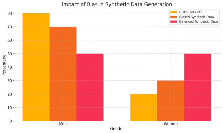
Similar to real data, synthetic data could also be susceptible to historical bias. Synthetic data might reproduce biases if it is generated too accurately from the real data. Data scientists need to account for bias when developing ML models to make sure the newly generated synthetic data is more representative of reality.
Example: Consider a synthetic dataset generated for a hiring algorithm based on historical employment data. If the historical data contains gender or racial biases (e.g., fewer women or minorities in certain roles), synthetic data generated from this dataset might perpetuate these biases.
Scenario: A synthetic dataset used to train a hiring algorithm might still reflect gender imbalances if it reproduces historical biases. Data scientists should ensure that the synthetic data includes diverse and balanced representations to avoid reinforcing existing biases. Techniques like re-weighting or augmenting the synthetic data to include a balanced representation of different groups can help address this issue.
Should be free from privacy concerns:
If the synthetic data generated from the real-world data are too similar, it can create the same privacy issues. When real-world data contains personal identifiers, then the synthetic data generated by it can also be subject to privacy regulations.
Example: Imagine a synthetic dataset is generated from medical records containing personal information. If the synthetic data is too similar to the original records, it could inadvertently reveal personal details, such as specific health conditions or treatments, which could still be traceable to individuals.
Scenario: A synthetic dataset for medical research that closely mimics real patient records might still have characteristics that could potentially identify individuals if not properly anonymized. To address this, the synthetic data should be generated with techniques that ensure the removal of any identifiable features and maintain privacy, such as differential privacy methods, which add noise to the data to prevent re-identification.
Case Studies and Industry Examples
Leveraging Industry Success Stories
One of the most compelling ways to understand the power of overcoming data scarcity is through real-world industry examples. These examples not only demonstrate the practical application of synthetic data and simulation techniques but also highlight the innovative approaches taken by leading companies to solve data challenges.
– Tesla: Simulated Driving Data
Tesla has pioneered the use of synthetic data to train its autonomous driving models. Instead of relying solely on vast amounts of real-world driving data, which can be expensive and time-consuming to collect, Tesla generates simulated driving scenarios. These simulations replicate a wide range of driving conditions, from different weather patterns to complex traffic situations. By using simulated data, Tesla can continuously improve its models, ensuring they perform safely and efficiently in the real world. This approach accelerates development and addresses the challenge of gathering sufficient data for rare or dangerous driving situations.
– Pharmaceutical Companies: Synthetic Data in Drug Discovery
In the pharmaceutical industry, the use of synthetic data has become a crucial tool in accelerating drug discovery. Traditional drug development relies heavily on real-world data, such as patient records and clinical trial results, which can be limited and difficult to obtain. By generating synthetic data that models drug interactions and patient responses, pharmaceutical companies can simulate the effects of new compounds before they even enter clinical trials. This approach speeds up the discovery process, reduces costs, and allows researchers to explore a broader range of potential treatments.
Key Lessons Learned from Industry Practices
Drawing from industry successes, several best practices stand out in the effort to overcome data scarcity. These lessons offer valuable insights for practitioners looking to apply similar strategies in their work.
1. Validation Against Real-World Data:
One crucial takeaway is the need to validate synthetic data against real-world data. Whether you’re using simulation-based methods like Tesla or generating synthetic data for pharmaceutical research, it’s essential to ensure that the synthetic data accurately represents the target domain. Validation ensures that the insights derived from models trained on synthetic data are credible and applicable in real-world scenarios. This step not only enhances the reliability of the models but also builds trust in the synthetic data approach.
2. Combining Multiple Techniques:
Another key lesson is the power of combining various data augmentation techniques. While synthetic data generation is a powerful tool, it has its limitations, such as the potential for introducing biases or inaccuracies. By integrating synthetic data with other methods—such as transfer learning and leveraging open datasets—you can mitigate these limitations. Transfer learning allows models to apply knowledge from one domain to another, while open datasets provide a broader base of real-world examples. Together, these techniques create a more robust training dataset, improving model performance and generalization.
Future Trends in Overcoming Data Scarcity
1. Automated Data Labeling:
Automated data labeling tools are becoming increasingly sophisticated, allowing for rapid annotation of large datasets with minimal human intervention. These tools often leverage AI to predict labels, which are then refined through a semi-supervised learning process. This trend is reducing the time and cost associated with creating large labeled datasets.
Examples:
AI-Driven Annotators:
Tools like Labelbox , LabelImg or Scale AI use AI to assist with the labeling process, enabling faster and more accurate annotations for tasks like object detection in images or sentiment analysis in text.
Zero-Shot and Few-Shot Learning Advances:
Zero-shot and few-shot learning are pushing the boundaries of what’s possible with limited data. In zero-shot learning, models are trained to recognize objects or concepts without having seen any labeled examples, relying on semantic information or transfer learning. Few-shot learning involves training models with only a few labeled examples, making it possible to deploy models in data-scarce environments.
Examples:
- Zero-Shot Learning with Flairs TARS Model:
In the context of zero-shot learning, where the goal is to classify text into categories that the model has not seen during training, pre-trained models like TARS can be highly effective. This means you can classify text without (m) any training examples.
The following code snippet illustrates how to use the TARS (Task-aware representation of sentences)model from the Flair library to perform zero-shot classification:
For instance, say you want to predict whether the text is “happy” or “sad” but you have no training data for this. Just use TARS with this snippet:
from flair.models import TARSClassifier
from flair.data import Sentence

# 1. Load our pre-trained TARS model for English
tars = TARSClassifier.load('tars-base')

# 2. Prepare a test sentence
sentence = Sentence("I am so glad you liked it!")

# 3. Define some classes that you want to predict using descriptive names
classes = ["happy", "sad"]

#4. Predict for these classes
tars.predict_zero_shot(sentence, classes)

# Print sentence with predicted labels
print(sentence)
Source:github.com/flairNLP/flair/blob/master/resources/docs/TUTORIAL_10_TRAINING_ZERO_SHOT_MODEL.md
- Few-Shot Learning with Prototypical Networks
Few-shot learning is particularly valuable in scenarios where labeled data is limited. By training models to recognize new object categories from just a few examples, we can effectively address data scarcity challenges. Below is an illustration of few-shot learning using Prototypical Networks, a popular method in this domain.
import torch
import torchvision
import torch.nn as nn
import torch.nn.functional as F
import torch.optim as optim
from torch.autograd import Variable
from tqdm import trange
from time import sleep
from sklearn.preprocessing import OneHotEncoder, LabelEncoder


class Net(nn.Module):
    """
    Image2Vector CNN which takes image of dimension (28x28x3) and return column vector length 64
    """

    def sub_block(self, in_channels, out_channels=64, kernel_size=3):
        block = torch.nn.Sequential(
            torch.nn.Conv2d(kernel_size=kernel_size, in_channels=in_channels,
                            out_channels=out_channels, padding=1),
            torch.nn.BatchNorm2d(out_channels),
            torch.nn.ReLU(),
            torch.nn.MaxPool2d(kernel_size=2)
        )
        return block

    def __init__(self):
        super(Net, self).__init__()
        self.convnet1 = self.sub_block(3)
        self.convnet2 = self.sub_block(64)
        self.convnet3 = self.sub_block(64)
        self.convnet4 = self.sub_block(64)

    def forward(self, x):
        x = self.convnet1(x)
        x = self.convnet2(x)
        x = self.convnet3(x)
        x = self.convnet4(x)
        x = torch.flatten(x, start_dim=1)
        return x


class PrototypicalNet(nn.Module):
    def __init__(self, use_gpu=False):
        super(PrototypicalNet, self).__init__()
        self.f = Net()
        self.gpu = use_gpu
        if self.gpu:
            self.f = self.f.cuda()

    def forward(self, datax, datay, Ns, Nc, Nq, total_classes):
        """
        Implementation of one episode in Prototypical Net
        datax: Training images
        datay: Corresponding labels of datax
        Nc: Number  of classes per episode
        Ns: Number of support data per class
        Nq:  Number of query data per class
        total_classes: Total classes in training set
        """
        k = total_classes.shape[0]
        K = np.random.choice(total_classes, Nc, replace=False)
        Query_x = torch.Tensor()
        if(self.gpu):
            Query_x = Query_x.cuda()
        Query_y = []
        Query_y_count = []
        centroid_per_class = {}
        class_label = {}
        label_encoding = 0
        for cls in K:
            S_cls, Q_cls = self.random_sample_cls(datax, datay, Ns, Nq, cls)
            centroid_per_class[cls] = self.get_centroid(S_cls, Nc)
            class_label[cls] = label_encoding
            label_encoding += 1
            # Joining all the query set together
            Query_x = torch.cat((Query_x, Q_cls), 0)
            Query_y += [cls]
            Query_y_count += [Q_cls.shape[0]]
        Query_y, Query_y_labels = self.get_query_y(
            Query_y, Query_y_count, class_label)
        Query_x = self.get_query_x(Query_x, centroid_per_class, Query_y_labels)
        return Query_x, Query_y

    def random_sample_cls(self, datax, datay, Ns, Nq, cls):
        """
        Randomly samples Ns examples as support set and Nq as Query set
        """
        data = datax[(datay == cls).nonzero()]
        perm = torch.randperm(data.shape[0])
        idx = perm[:Ns]
        S_cls = data[idx]
        idx = perm[Ns: Ns+Nq]
        Q_cls = data[idx]
        if self.gpu:
            S_cls = S_cls.cuda()
            Q_cls = Q_cls.cuda()
        return S_cls, Q_cls

    def get_centroid(self, S_cls, Nc):
        """
        Returns a centroid vector of support set for a class
        """
        return torch.sum(self.f(S_cls), 0).unsqueeze(1).transpose(0, 1) / Nc

    def get_query_y(self, Qy, Qyc, class_label):
        """
        Returns labeled representation of classes of Query set and a list of labels.
        """
        labels = []
        m = len(Qy)
        for i in range(m):
            labels += [Qy[i]] * Qyc[i]
        labels = np.array(labels).reshape(len(labels), 1)
        label_encoder = LabelEncoder()
        Query_y = torch.Tensor(
            label_encoder.fit_transform(labels).astype(int)).long()
        if self.gpu:
            Query_y = Query_y.cuda()
        Query_y_labels = np.unique(labels)
        return Query_y, Query_y_labels

    def get_centroid_matrix(self, centroid_per_class, Query_y_labels):
        """
        Returns the centroid matrix where each column is a centroid of a class.
        """
        centroid_matrix = torch.Tensor()
        if(self.gpu):
            centroid_matrix = centroid_matrix.cuda()
        for label in Query_y_labels:
            centroid_matrix = torch.cat(
                (centroid_matrix, centroid_per_class[label]))
        if self.gpu:
            centroid_matrix = centroid_matrix.cuda()
        return centroid_matrix

    def get_query_x(self, Query_x, centroid_per_class, Query_y_labels):
        """
        Returns distance matrix from each Query image to each centroid.
        """
        centroid_matrix = self.get_centroid_matrix(
            centroid_per_class, Query_y_labels)
        Query_x = self.f(Query_x)
        m = Query_x.size(0)
        n = centroid_matrix.size(0)
        # The below expressions expand both the matrices such that they become compatible to each other in order to caclulate L2 distance.
        # Expanding centroid matrix to "m".
        centroid_matrix = centroid_matrix.expand(
            m, centroid_matrix.size(0), centroid_matrix.size(1))
        Query_matrix = Query_x.expand(n, Query_x.size(0), Query_x.size(
            1)).transpose(0, 1)  # Expanding Query matrix "n" times
        Qx = torch.pairwise_distance(centroid_matrix.transpose(
            1, 2), Query_matrix.transpose(1, 2))
        return Qx


def train_step(protonet, datax, datay, Ns, Nc, Nq):
    optimizer.zero_grad()
    Qx, Qy = protonet(datax, datay, Ns, Nc, Nq, np.unique(datay))
    pred = torch.log_softmax(Qx, dim=-1)
    loss = F.nll_loss(pred, Qy)
    loss.backward()
    optimizer.step()
    acc = torch.mean((torch.argmax(pred, 1) == Qy).float())
    return loss, acc


def test_step(protonet, datax, datay, Ns, Nc, Nq):
    Qx, Qy = protonet(datax, datay, Ns, Nc, Nq, np.unique(datay))
    pred = torch.log_softmax(Qx, dim=-1)
    loss = F.nll_loss(pred, Qy)
    acc = torch.mean((torch.argmax(pred, 1) == Qy).float())
    return loss, acc


def load_weights(filename, protonet, use_gpu):
    if use_gpu:
        protonet.load_state_dict(torch.load(filename))
    else:
        protonet.load_state_dict(torch.load(filename), map_location='cpu')
    return protonet
Source:github.com/Hsankesara/DeepResearch/blob/master/Prototypical_Nets/prototypicalNet.py
This implementation of Prototypical Networks in PyTorch includes the necessary components for training and evaluating the model. The code defines the network architecture, including a convolutional neural network for feature extraction and the Prototypical Network for few-shot classification.
Conclusion
Data scarcity is a critical challenge in AI development, as it directly impacts the ability of models to learn, generalize, and make accurate predictions. So at IOSCAPE, we are trying to overcome these challenges which require innovative techniques, such as data augmentation, synthetic data generation, transfer learning, and few-shot learning, which can help mitigate the effects of limited data and enable the development of robust AI systems even in data-constrained environments.